Integrating Domain Knowledge in Data-driven Earth Observation with Process Convolution

Daniel Heestermans Svendsen, Maria Piles, Jordi Muñoz-Marí, David Luengo, Luca Martino and Gustau Camps-Valls

The modelling of Earth observation data is a challenging problem, typically approached by either purely mechanistic or purely data-driven methods. Mechanistic models encode the domain knowledge and physical rules governing the system. Such models, however, need the correct specification of all interactions between variables in the problem and the appropriate parameterization is a challenge in itself. On the other hand, machine learning approaches are flexible data-driven tools, able to approximate arbitrarily complex functions, but lack interpretability and struggle when data is scarce or in extrapolation regimes. In this paper, we argue that hybrid learning schemes that combine both approaches can address all these issues efficiently. We introduce Gaussian process (GP convolution models for hybrid modelling in Earth observation (EO) problems. We specifically propose the use of a class of GP convolution models called latent force models (LFMs) for EO time series modelling, analysis and understanding. LFMs are hybrid models that incorporate physical knowledge encoded in differential equations into a multioutput GP model. LFMs can transfer information across time-series, cope with missing observations, infer explicit latent functions forcing the system, and learn parameterizations which are very helpful for system analysis and interpretability. We illustrate the performance in two case studies. First, we consider time series of soil moisture from active (ASCAT) and passive (SMOS, AMSR2) microwave satellites. We show how assuming a first order differential equation as governing equation, the model automatically estimates the e-folding time or decay rate related to soil moisture persistence and discovers latent forces related to precipitation. In the second case study, we show how the model can fill in gaps of leaf area index (LAI) and Fraction of Absorbed Photosynthetically Active Radiation (fAPAR) from MODIS optical time series by exploiting their relations across different spatial and temporal domains. The proposed hybrid methodology reconciles the two main approaches in remote sensing parameter estimation by blending statistical learning and mechanistic modeling.

We provide the code for the implementation of the Latent Force Model with a 1st order ODE kernel as well as a notebook showing the modelling of the timeseries of soil moisture products SMOS, ASCAT and AMSR2.

Latent force models as a hybrid between purely mechanistic and purely statistical methods

Latent Force Models (LFMs) are a way to encode knowledge of the governing equations of a system of interest into GP regression. This blog post aims to present the model as hybrid approach, neither purely physics-based nor purely statistical.

As described in the paper, we assume that the signals you are observing $y_q(t)$ are governed by an underlying ordinary differential equation (ODE) with one or more Gaussian process latent forcings. We follow the procedure described in (Alvarez et al. 2009) which shows that the solution to the ODE is itself a Gaussian process over the outputs with a multi-output kernel which contains parameters of the underlying ODE.

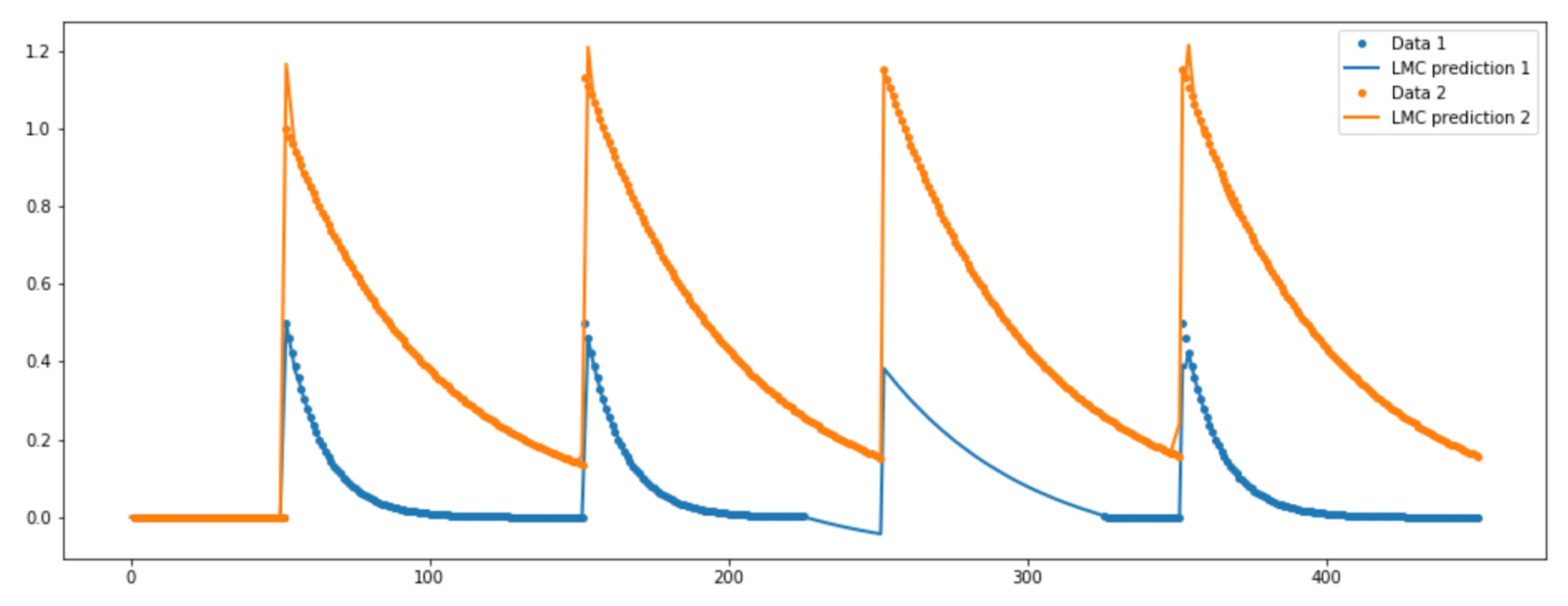
The LFM lends from both the physics-based and statistical approaches. Consider a synthetic dataset generated by a 1st order ODE governing two signals that are linked to the same latent force. We remove the data from one of the time series between the values of t=225 and t=325 to illustrate how this approach copes with missing data. The latent force is a superposition of delta-functions at $t=50, 150, 250$ and $350$.

Let us try a fully physics-based approach beginning from the analytical solution to the 1st order inhomogeneous ODE:

$y_q(t) = \frac{B_q}{D_q} + \sum_{r=1}^R S_{rq} \exp(-D_q t) \int_0^t f_r(\tau ) \exp (D_q \tau ) d \tau$

Since the latent force $f$ is unknown we can discretize the integral above, splitting $f$ into discrete values which one could fit by minimizing some cost function. For this, we can compute the squared loss between this purely theoretical solution and find the parameters minimizing the error. Below we see the fit of the two signals on the left and the fit of the latent forces on the right.

We note that the mechanistic model fits the data nicely and does very well in interpolating the gap. It also fits the latent force very well, up to a multiplicative constant which we also saw for the LFM. The LFM does similarly well in this problem as shown below

As a purely statistical approach we chose the Linear Model of Coregionalization (LMC). The figure below shows the LMC does not do as well as the LFM or the purely mechanistic model despite trying different kernel functions. The LMC and the LFM are essentially the same model (a multi-output GP) using two different multi-output kernel functions.

The conclusion is of course that the function is very hard to model, due to its many discontinuities, unless we use a prior over the function that is a good fit (which we can do in the case of the mechanistic model or the LFM). In the shown examples we are able to obtain a good fit since we derived the kernel for the GP prior from the underlying governing equations.

The mechanistic approach described above does not work well outside synthetic experiments, however, because it is too faithful to the analytical solution of the ODE and, as described in our paper (link to come), when the 1st order ODE is only an approximation to the system, this apporach does poorly. The LFM, however, can model noise and is more flexible, and leads to inference of physically meaning parameters and latent forces. In this way the LFM combines the best of both worlds.

$.$